
Introduction
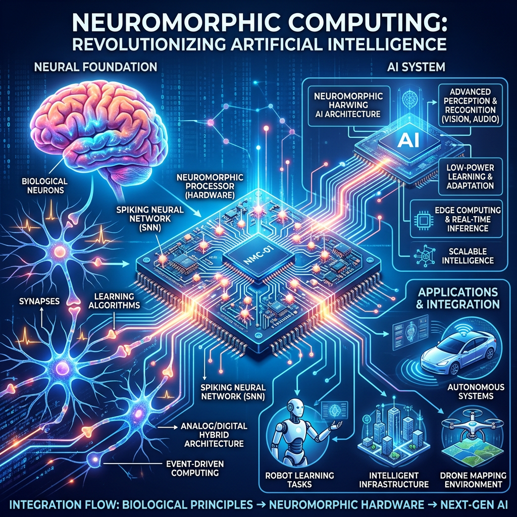
This post introduces Neuromorphic Computing and describes how this development will be integrated into the field of Artificial Intelligence (AI).
It is interesting for me to look back at the field of study I chose in the 1980s: Electrical Engineering. I spent the subsequent decades working in Software and Data Engineering, but developments in AI are now compelling me to return to that domain.
A number of experts now agree that the current massive investments in AI will not continue in their present form.
Why not? Large Language Models (LLMs) will undergo further development and refinement, but they are not the solution to Artificial General Intelligence (AGI).
New types of models are already being developed, yet these, too, are unlikely to yield the desired result.
Meanwhile, the development of the ecosystem surrounding these models—including generative AI, AI agents, hardware architectures, and so on—will naturally continue unabated.
We are now about to take a remarkable turn: towards a brain-inspired approach to building computers, whereas existing AI is based mostly on data and (statistical) algorithms capable of performing intelligent tasks.
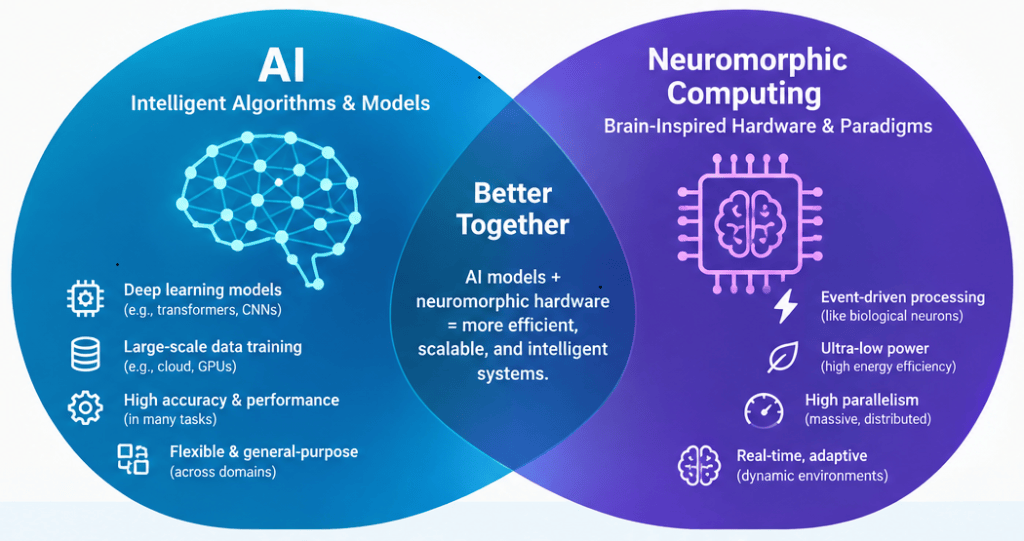
As this topic diverges significantly from mainstream AI developments, it will be the subject of several subsequent posts.
Below is a brief list of the topics that will be covered:
- Hardware fundamentals of Neuromorphic Computing
- What is Neuromorphic Computing?
- Current applications of the Neural Processing Unit (NPU)
- Neuromorphic local learning rules
- Neuromorphic Quantum Computing
- Convergence of Neuroscience, AGI, and Neuromorphic Computing
To fully understand this topic, we must first return to the basic electrical components. If you are not familiar with this field, you may skip the next section “Hardware Fundamentals of Neuromorphic Computing”.
The section “What is Neuromorphic Computing?” explains how computer systems are designed to mimic the structure and function of the human brain.
The last section in this post “Applications of the NPU”, describes the applications of the currently available processing units and how they complement each other today.
Hardware Fundamentals of Neuromorphic Computing
The memristor forms the basis for Neuromorphic Computing, due to the following properties:
- Charge-dependent resistance
- Memory retention when the power supply is disconnected
- Low power consumption
- Support for in-memory learning
The following paragraphs in this section describe basic electrical components, including the memristor and memristor crossbar arrays, and how memristors differ from GPUs.
Basic Electrical Components
The figure below shows the theoretical symmetry between the non-linear resistor (voltage vs. current), non-linear capacitor (voltage vs. charge), and non-linear inductor (magnetic flux linkage vs. current).
From this symmetry, the characteristics of a fourth fundamental non-linear circuit element can be deduced, linking magnetic flux and charge, which is called the memristor (interweaving of memory and resistor)1. In contrast to a linear (or non-linear) resistor, the memristor has a dynamic relationship between current and voltage, including a memory of past voltages or currents.
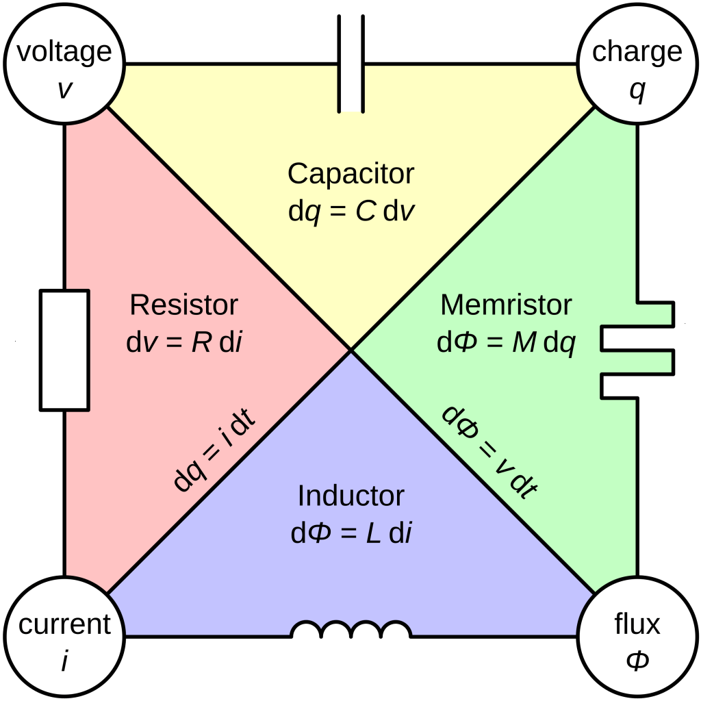
Basic Characteristics of the Memristor
The memristance function describing the charge-dependent rate of change of magnetic flux with charge is
Substituting the flux as the time integral of the voltage, and charge as the time integral of current, the more convenient forms are
| Device | Symbol | Characteristic property | Units | Unit ratio (V, A, C, Wb) | Differential equation |
|---|---|---|---|---|---|
| Resistor | R | Resistance | ohm (Ω) | volts per ampere (V / A) | R = dV / dI |
| Capacitor | C | Capacitance | farad (F) | coulombs per volt (C / V) | C = dq / dV |
| Inductor | L | Inductance | henry (H) | webers per ampere (Wb / A) | L = dΦm / dI |
| Memristor | M | Memristance | ohm (Ω) | webers per coulomb (Wb / C) | M = dΦm / dq |
If M(x) is a constant function (i.e. has the same value for all x), then we obtain Ohm’s law: R(t) = V(t)/I(t). If M(x) is nontrivial, however, the equation is not equivalent because q(t) and thus M(q(t)) varies with time. Solving for voltage as a function of time produces
This equation reveals that memristance defines a linear relationship between current and voltage, as long as M does not vary with charge.
Non-zero direct current (DC) implies time-varying charge. Alternating current (AC), however, may reveal the linear dependence in circuit operation by inducing a measurable voltage without net charge movement. This holds as long as the maximum value of q does not cause much change in M compared to the initial value M(0).
→ This is why memristance is charge-dependent resistance.
Furthermore, the memristor has a constant memristance if no current is applied. So, if I(t) = 0, M(q(t)) is constant due to q(t) being constant.
→ This is the essence of the memory effect.
The power consumption characteristic recalls that of a resistor, I2R:
As long as M(q(t)) varies little, such as under AC, the memristor will appear as a constant resistor. If M(q(t)) increases rapidly, however, current and power consumption will quickly stop.
→ This is why memristor learning consumes orders of magnitude less energy than GPU training.
Memristor Crossbar Array
A memristive crossbar array consists of two sets of perpendicular conducting wires—rows and columns—forming a grid. At each intersection, a memristor bridges the row and column, allowing current to flow depending on its programmed memristance.
Before proceeding, we must first define conductance in the context of the memristor: by analogy with memristance, we can define W(ϕ(t)) as memductance (interweaving of memory and conductance)
Memductance with respect to flux is the inverse of memristance with respect to charge, and therefore the unit of memductance is the same as the unit of conductance – siemens (S or Ω−1).
Now we can look at memristor crossbars, which compute as follows
where G is the conductance matrix, in which the synaptic weights are stored. Crossbar arrays exploit Ohm’s and Kirchhoff’s laws:
This means applying voltages to rows produces column currents equal to a matrix‑vector multiplication. Parallel analog computation is enabled, reducing the need to transfer data between memory and processor.
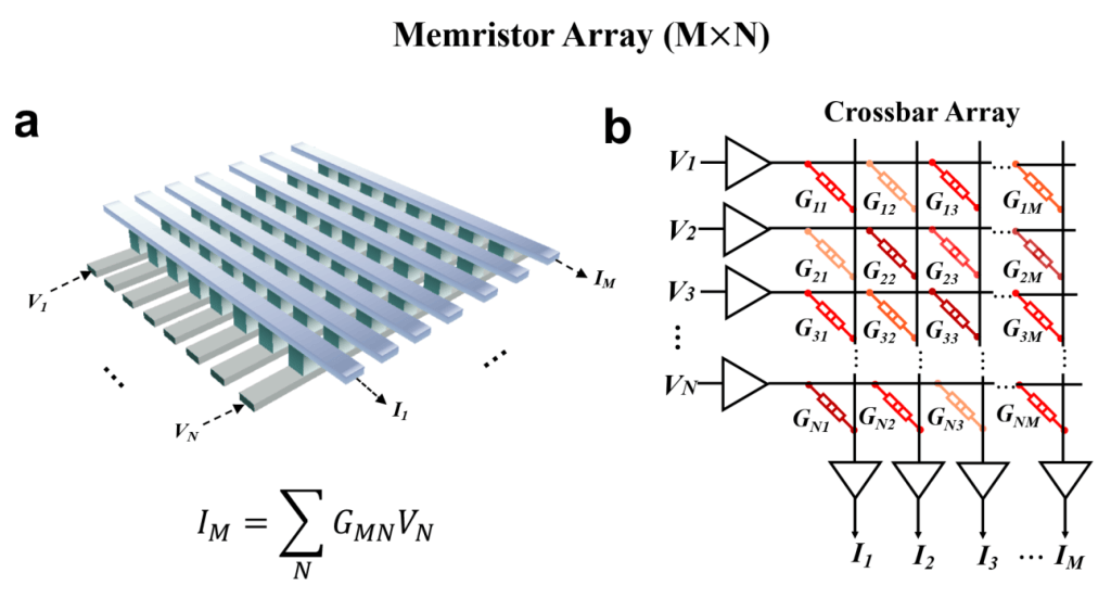
→ This is why memristors are used in physical neural networks and in‑memory computing.
How Memristors differ from GPUs
A GPU separates compute (matrix multiplications) from memory (VRAM). Every training step requires shuttling huge tensors back and forth, the von Neumann bottleneck.
Memristors break this separation, because they can merge the functionality of the arithmetic logic unit and the memory unit without data transfer.
A memristor stores a weight and performs the multiply‑accumulate operation in the same physical location. This is what in-memory learning means.
The following is a summary of how learning happens without GPUs:
- Store weights as resistances. Each memristor’s resistance encodes a synaptic weight
- Compute using Ohm’s law. Applying voltages across a crossbar produces currents equal to weighted sums. This is analog matrix multiplication performed in place
- Update weights by applying pulses. Local learning rules—Hebbian, Spike-Time-Dependent Plasticity (STDP), and gradient‑based approximations—are implemented by sending electrical pulses that shift oxygen vacancies or domain walls. This directly modifies the resistance
- No data movement. Because the weight lives in the device that performs the computation, there is:
- no VRAM
- no PCI bottleneck
- no GPU memory hierarchy
- no tensor shuttling, the compute is the memory
In summary, memristors enable the following:
- On‑chip learning (no GPU)
- Ultra‑low‑power continual learning
- Real‑time sensorimotor loops
- Massively parallel analog computation
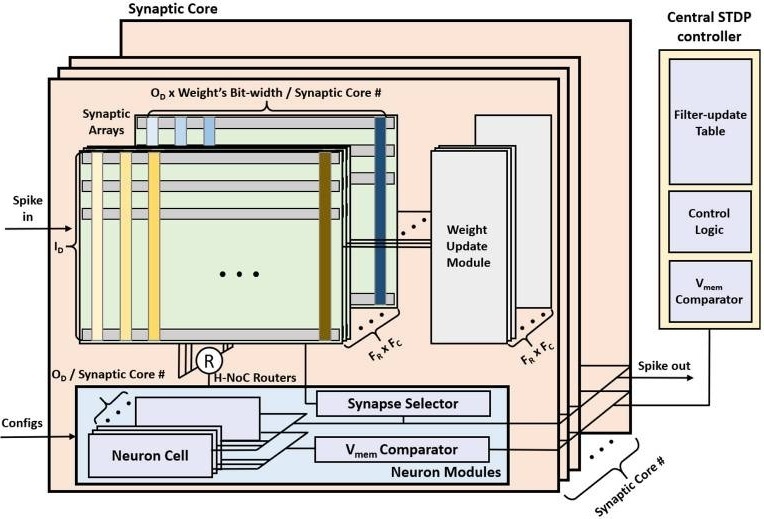
- Brain‑like architectures (Loihi, Akida, MoNETA)
MoNETA is an example of a whole‑brain model running on memristive hardware.
What is Neuromorphic Computing?
Neuromorphic Computing is a way of building computers inspired by the human brain that merges memory and processing, uses spiking neurons, and delivers massive efficiency gains for AI‑like tasks.
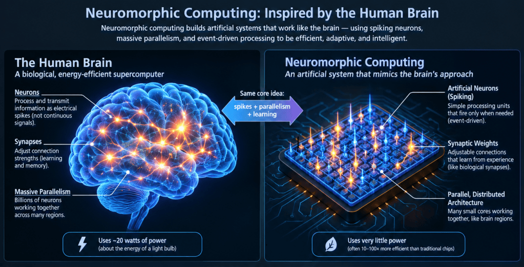
The following paragraphs in this section explain why Neuromorphic systems exist, how they work, and where they are used.
Why Neuromorphic Systems exist
Traditional computers follow the von Neumann architecture, where the processor and memory are physically separate. This creates a bottleneck because data must constantly shuttle back and forth between them, consuming time and energy, especially in AI workloads. Every time the processor needs data, it has to fetch it from memory, do something with it, and send results back.
As AI models grow, this bottleneck becomes worse, requiring billions of memory lookups during training.
Neuromorphic systems solve this by bringing memory and processing together in one place, just as biological neural tissue in the human brain does.
How Neuromorphic Systems work
The image below illustrates how Neuromorphic systems work and the process flow it goes through.
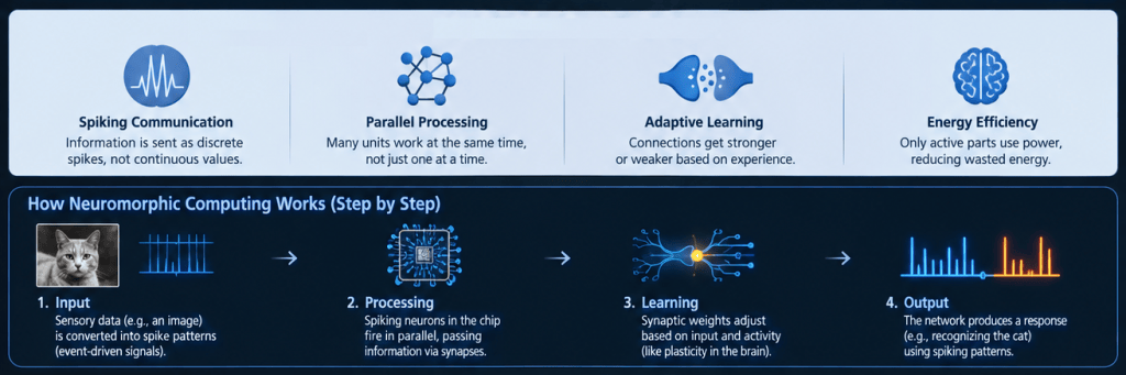
Neuromorphic systems are designed to replicate the human brain’s cognitive functions, such as perception, learning, reasoning, and problem-solving. They utilize AI and machine learning algorithms to process data and make decisions.
Hardware Implementation of Neuromorphic Systems
→ Co‑located memory and computation
The brain doesn’t have a separate memory warehouse; learning and processing happen in the same tissue. Neuromorphic systems replicate this by using on‑chip memory tightly integrated with computation.
→ Spiking Neural Networks (SNNs)
Instead of passing continuous numbers like standard AI, Neuromorphic systems use electrical spikes, mimicking biological neurons and they process information through SNNs, which communicate in discrete electrical spikes rather than the continuous streams of numbers used by standard AI systems.
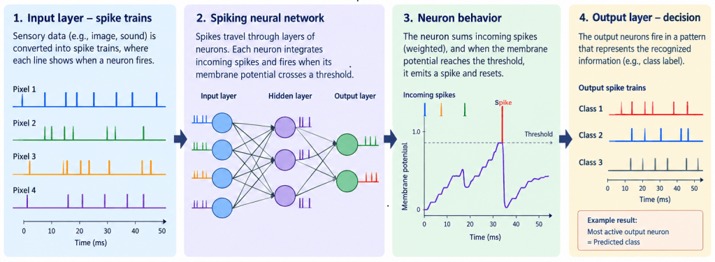
Spikes are sparse and energy‑efficient, neurons fire only when needed, not continuously.
→ Temporal coding
Information is encoded not just in how often a neuron fires, but when it fires relative to others. This makes computation far more efficient than conventional deep learning, which processes dense batches of numbers.
The figure below summarizes the key mechanisms in a SNN.

An example Python program that simulates a brain-like cell can be found as an attachment at the end of the post.
Why Neuromorphic Computing is powerful
Neuromorphic chips can be orders of magnitude more energy‑efficient than conventional processors. For example, advanced Neuromorphic transistor designs achieve energy consumption per spike ~80× lower than standard silicon at similar scales.
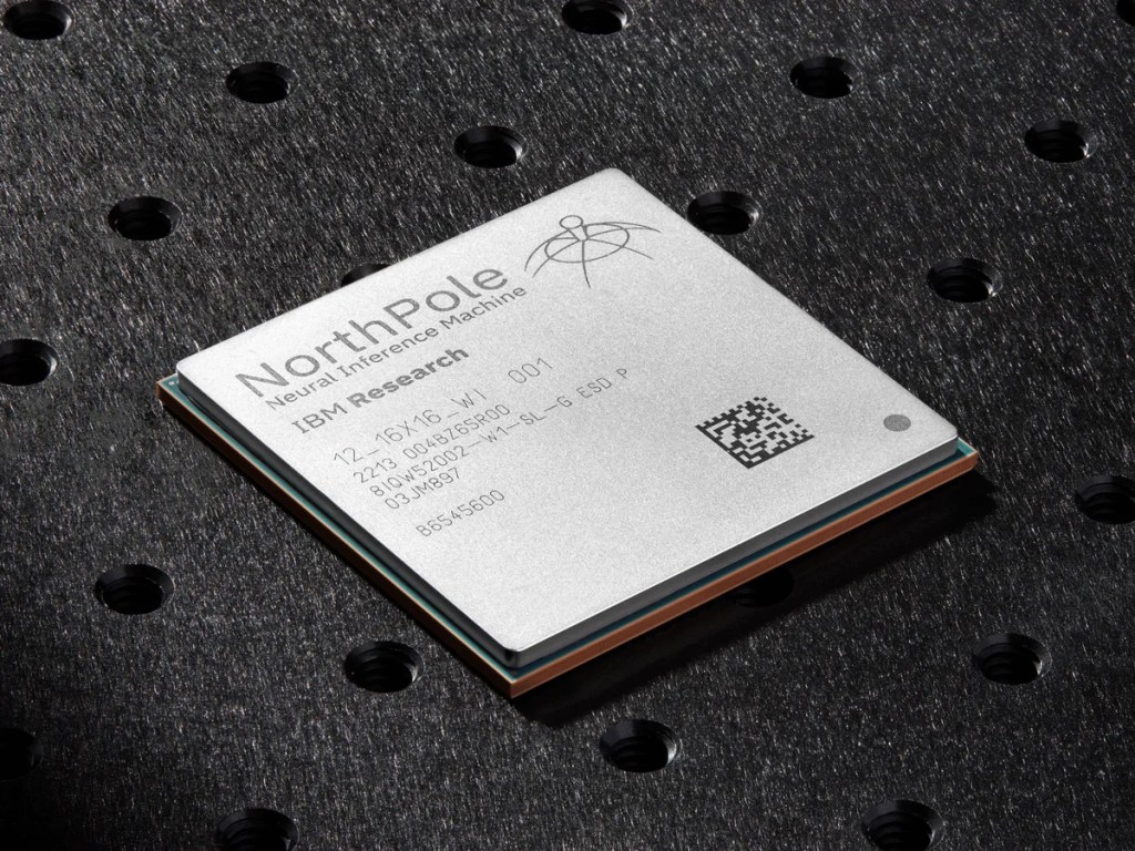
IBM’s NorthPole chip is 25× more energy efficient than leading conventional chips and achieves its speed by eliminating the memory‑shuttling bottleneck entirely.
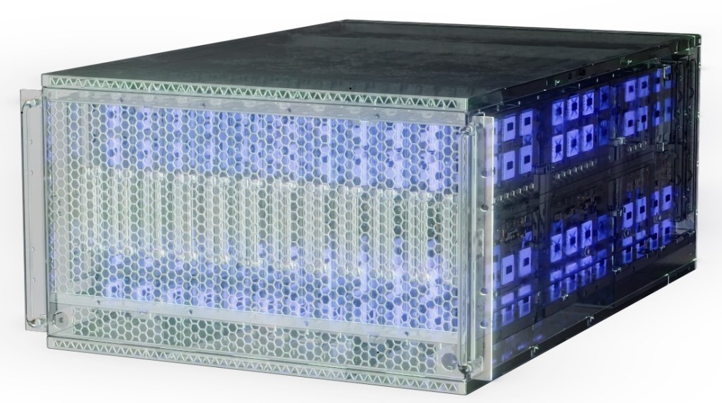
Hala Point is Intel’s largest and, to date, most advanced Neuromorphic system for more sustainable AI. The system houses 1,152 Loihi 2 processors produced using the Intel 3 process within a six-rack-unit chassis. It supports up to 1.15 billion neurons and 128 billion synapses distributed over 140,544 Neuromorphic processing cores, with a power consumption of 2,600 watts. Additionally, it features over 2,300 embedded x86 processors for ancillary computations.
Where Neuromorphic Computing is used
Neuromorphic systems excel in edge computing, where low power and fast local decision‑making matter:
- Autonomous systems
- Event‑based vision systems
- Speech recognition and keyword spotting
- Biomedical signal processing
The market is projected to grow from $7.5B in 2026 to $35B in 2036 (16.5% CAGR)
What Neuromorphic Computing is NOT
Neuromorphic systems do not replace general‑purpose computers. They are not suited for spreadsheets, databases, or typical software workloads.
Their strength is narrow but dramatic: fast, efficient, brain‑like processing of sensory and temporal data.
Applications of the NPU
In this final section of the post, we explain where we currently stand with Neuromorphic Computing and its applications.
Nowadays, Neuromorphic Computing is primarily used in NPUs. These AI accelerators are found in the following devices for edge AI applications:
- Autonomous vehicles, drones, and robots
- Smart cameras and security systems
- Wearable devices
- Smart home appliances
- Industrial IoT
- Healthcare devices such as EEG and ECG
NPUs are inference‑focused:
- NPUs are designed for real‑time, on‑device AI, because they enable on-device generative AI apps capable of processing AI applications with relatively low power consumption
- NPUs use low‑precision arithmetic, supporting 8‑bit (or lower) operations to increase efficiency
- NPUs integrate synaptic weights for fast local computation, by performing storage and computation on-chip
- NPUs are used in smartphones, laptops, IoT devices. These are inference workloads
- NPUs accelerate LLM inference, becasue they offer dramatic improvements in tasks like speech recognition and natural language generation
NPUs do not train large models:
- Training LLMs requires massive memory bandwidth, typically hundreds of GB/s to TB/s bandwidth and tens to hundreds of GB of memory. NPUs have small on‑chip memory optimized for fast reuse, not large model storage
- Training requires high precision, using FP16/BF16/FP32. NPUs use INT8 or lower for efficiency
- Training requires huge compute clusters, so LLMs are trained on GPU/TPU clusters, not on NPUs
- NPUs are designed for edge computing, i.e. they are ideal for edge AI and on-device AI with low power consumption
| Task | NPU | GPU/TPU |
|---|---|---|
| Train large models | ❌ Not suitable | ✅ Primary use |
| Fine‑tune small models | ⚠️ Possible but limited | ✅ Common |
| Run inference | ✅ Ideal | ✅ Also common |
| On-device AI | ⭐ Best fit | ❌ Too power-hungry |
Conclusion
This post describes the basic principles of Neuromorphic Computing, based on the memristor:
- Hardware fundamentals of Neuromorphic Computing
- Overview of Neuromorphic Computing
- Applications of Neuromorphic Computing in the NPU
Finally, the current state of Neuromorphic Computing is described, along with its limitations and the areas where further development is needed.
At present, therefore, Neuromorphic Computing remains a technology that complements existing ones.
The topic will be explored further in future posts, as will its potential integration into AGI.
Glossary of Terms
- AC – Alternating current is an electric current that periodically reverses direction and changes its magnitude continuously with time
- AGI – Artificial General Intelligence, refers to a type of AI that aims to replicate human cognitive abilities
- AI accelerator – a specialized processor—such as a GPU, TPU, or NPU—designed to speed up AI workloads by performing massive parallel matrix and tensor computations far faster and more efficiently than a CPU
- CAGR – Compound Annual Growth Rate, representing the average annual growth of an investment
- Charge (electric) – fundamental property of matter, existing in two types—positive and negative—and quantified in units of coulombs (C)
- Chip – an integrated circuit (IC) built upon a tiny wafer of silicon
- Conductance – the measure of how easily electric current flows through a material, and it is the reciprocal of resistance, measured in siemens (S)
- CPU – Central Processing Unit, an electronic circuit designed for executing instructions and managing operations
- Crossbar array – a rectilinear architecture where each crosspoint hosts a nanoscale device (memristor) whose conductance can be programmed. This structure supports in‑memory computing, Neuromorphic processing, and high‑density non‑volatile memory
- DC – Direct current flows in a constant direction, distinguishing it from AC
- Deep learning – a subset of machine learning that uses multilayered neural networks to simulate the complex decision-making power of the human brain
- Edge AI – the deployment of AI directly on local devices, enabling real-time data processing and decision-making without relying on cloud servers
- ECG – Electrocardiography, the process to record an electrocardiogram of the heart’s electrical activity through repeated cardiac cycles
- EEG – Electroencephalography, the process to record an electrogram of the spontaneous electrical activity of the brain
- Electric field – a vector field surrounding electric charges, defined as the force per unit positive charge E
- Flux (magnetic) – the measure of the total magnetic field Φ passing through a given surface, quantified in webers (Wb)
- GPU – Graphics Processing Unit, a specialized electronic circuit designed to accelerate image processing and parallel computations
- Hebbean learning – involves Neuromorphic local learning from the activity of a group of neurons
- Kirchhoff’s laws – the Current Law (KCL), stating that the sum of currents entering a junction equals the sum leaving it, and the Voltage Law (KVL), stating that the sum of voltages around any closed loop is zero
- Magnetic field – an invisible vector field that exerts forces on moving electric charges and magnetic materials, generated by magnets or moving electric currents
- Memristor – a non-linear two-terminal electrical component relating electrical charge and magnetic flux linkage
- Neuron – a nerve cell that is excitable, firing electric signals called action potentials
- Neuroscience – the scientific study of the nervous system, exploring how neurons, glia, and neural circuits give rise to behavior, cognition, and consciousness
- NPU – Neural Processing Unit, a specialized computer microprocessor designed to mimic the processing function of the human brain
- Ohm’s law – the current (I) through a conductor is directly proportional to the voltage (V) across it and inversely proportional to its resistance R, expressed as V=IR
- Resistance – the property of a material or circuit that opposes the flow of electric current, measured in ohms (Ω) and defined by Ohm’s law
- Sensorimotor – refers to the integration of sensory experiences and motor actions, particularly in early childhood development, where infants learn about the world through their senses and movements
- STDP – Spike-Time-Dependent Plasticity, involves Neuromorphic local learning based on the timing of neural spikes and is used to modify synaptic connections on the precise timing of these spikes
- Synaptic weight – refers to the strength or amplitude of a connection between two nodes, corresponding in biology to the amount of influence the firing of one neuron has on another
- Tensor – a fundamental data structure used to represent and manipulate data
- TPU – Tensor Processing Unit, a specialized computer chip developed by Google to accelerate machine learning tasks, particularly deep learning, by efficiently processing large-scale tensor operations
- VRAM – Video Random Access Memory
References
- Memristor – The missing circuit element, Leon Chua, September 1971 ↩︎
- Two-terminal non-linear circuit elements, Parcly Taxel, 27 September 2013
↩︎ - The MONETA system architecture overview, Kim, Chakraborty, She, Lee, Kang and Mukhopadhyay, April 2022 ↩︎
- A new chip architecture points to faster, more energy-efficient AI, Mike Murphy, 19 October 2023 ↩︎
- Intel builds world’s largest Neuromorphic system, Mike Davies, 17 April 2024 ↩︎
- AI Chips Explained: GPU vs NPU vs TPU, Murali Teja, 24 July 2026 ↩︎
Attachments
A tiny simulation of a brain-like cell using the Brian2 Python library:
from brian2 import *start_scope()tau = 10*mseqs = '''dv/dt = (1.0 - v)/tau : 1'''G = NeuronGroup(1, eqs, threshold='v>1', reset='v = 0', method='exact')M = StateMonitor(G, 'v', record=0)run(100*ms)plot(M.t/ms, M.v[0])
This code simulates how a single neuron behaves. The neuron’s voltage rises slowly, and once it crosses a limit, it “fires” and then resets, just like a brain cell. This shows the basic idea behind Neuromorphic Computing: processing information the way our brains do.
 inteso.ai - blog
Leave a comment