Understanding Quantum Data Processing in Shor’s Algorithm

Introduction

In a previous post the concept of parallelism in a quantum circuit$^{[1]}$ is explained and below is a short recap.

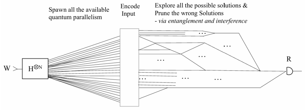
A typical quantum algorithm starts with a WRITE operation. It initializes all $n$ qubits in the input register in a base state. This is followed by the parallel spawning of quantum threads by applying $n$ Hadamard ($H$) gates. It results in $2^n$ quantum threads executing in parallel. Subsequently, the input data is encoded, typically in the quantum state’s amplitudes and phases. Execution of the algorithm then occurs in superposition and by parallel processing. During this process, probabilities are decreased by canceling out threads. Finally, a READ operation (measurement) of the output register is performed.

This flow description doesn’t explain how data plays a role during execution of the algorithm. The following data operations can be distinguished:

• Encoding the input register from classical bit strings
• Accessing Quantum Random Access Memory (QRAM)
• Measuring the output register

The first two items will be discussed at a later stage, when Quantum Machine Learning (QML) is addressed. This article focuses on how to process the output results of a quantum algorithm. This is not so straight forward as it seems. The information held in the output register can not directly be read into a classical bit string. As soon as qubits in superposition are measured, the superposition is destroyed. This implies that all information stored in the qubit amplitudes is lost. It only yields a classical outcome according to the probability distribution of the quantum state.

The next sections describe the only method to retrieve the algorithm’s outcome. The solution is the opposite of what is expected, because the input register is measured and not the output register. For this purpose, the following properties of quantum mechanics are used:

• Entanglement
• Interference

Shor’s algorithm is used as example to explain how these properties are applied.

Period finding in Shor’s algorithm

The algorithm is executed in a hybrid system. The pre- and post-processing parts are performed in a classical circuit. The period-finding part, or quantum part, is performed in a quantum circuit. In our example, $N = 33$ is the number to be factorized.

Pre-processing

Find a random number $a$ that is co-prime with $N$, i.e. $gcd(a, N) = 1$. In this case we choose $a = 5$.

Quantum register initialization

• Input register: superposition of all qubits in $x$
• Output register: result of calculation $f(x) = 5^x \bmod 33$

The input register is put in superposition:

Where $Q = 2^{n}$ and $n$ is the register size.

At this stage, there is no entanglement yet.

Algorithm execution

The algorithm calculates:

$5^1 \equiv 5 \bmod 33 \\5^2 \equiv 25 \bmod 33 \\5^3 \equiv 125 \equiv 26 \bmod 33 \\5^4 \equiv 26 \cdot 5 = 130 \equiv 31 \bmod 33 \\5^5 \equiv 31 \cdot 5 = 155 \equiv 23 \bmod 33 \\5^6 \equiv 23 \cdot 5 = 115 \equiv 16 \bmod 33 \\5^7 \equiv 16 \cdot 5 = 80 \equiv 14 \bmod 33 \\5^8 \equiv 14 \cdot 5 = 70 \equiv 4 \bmod 33 \\ 5^9 \equiv 4 \cdot 5 = 20 \bmod 33 \\5^{10} \equiv 20 \cdot 5 = 100 \equiv 1 \bmod 33\\5^{11} \equiv 1 \cdot 5 = 5 \bmod 33\\5^{12} \equiv 5 \cdot 5 = 25 \bmod 33\\\dots$

So, the smallest $r$ satisfying $5^r \equiv 1 \bmod 33$ is

$r = 10$

And that is exactly the period the quantum part is trying to find. The next steps in the quantum part describe entanglement and interference, needed for propagating the outcome of the algorithm.

Entanglement by algorithm execution

After execution of the algorithm, the input register state is:

And this is entangled, because:

• Different values of $x$ ​​share the same function value
• The registers are no longer separable in a product state

For example

$f(0) = 1 \\f(10) = 1\\f(20)=1\\\dots$

So, all $|0\rangle, |10\rangle, |20\rangle, \dots$in the input register are linked to the same $|1\rangle$ in the output register.

This back propagation of output to input makes the next step possible.

Interference by Fourier transform

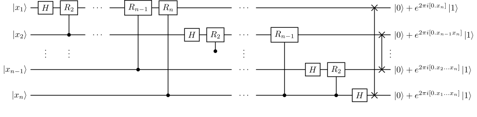
Quantum Fourier Transform (QFT) is applied to the input register. The QFT ensures that the amplitudes of the states corresponding to the period $r$ interfere constructively. The amplitude of the other states interfere destructively. Note that the QFT is applied to a regular pattern in the outcome of the period-finding algorithm.

Below is the quantum circuit$^{[2]}$ implementation for register size $n$. The circuit is composed of Hadamard ($H$) gates and the controlled version of dyadic rational phase ($R_k$) gates.

In our example, the result of the QFT is that the input register states with value

$k \cdot \frac{Q}{r}, \quad k = 1,2,3,\dots$

Get the highest probability. In the example of $Q = 2048$ ($Q \ge N^2$) and $r = 10$, the states with the highest probability are:

$\approx 205, 410, 614, \dots$

Finally, measuring of the algorithm result is possible.

Measurement Quantum part result

The input register is measured and the resulting bit string is probably:

$11001101$

And that is $205$ in decimal form. Repetition of the quantum part is needed, in case the measurement result is unreliable.

Post-processing

The quantum part yields $m = 205$ and the post-processing part calculates the prime factors in a classical way:

$\frac{m}{Q} \approx \frac{k}{r}$

And with a fraction approach (continued fractions), the result is $\frac{k}{10}$ and hence $r = 10$

The following formulas yield the prime factors:

$\gcd\left(a^{r/2} – 1, N\right), \quad \gcd\left(a^{r/2} + 1, N\right)$

$a^{r/2} = 5^{5} = 3125 \equiv 23 \bmod 33$

Hence

$\gcd(23 – 1, 33) = \gcd(22, 33) = 11,\quad\gcd(23 + 1, 33) = \gcd(24, 33) = 3$

Final result: the prime factors of 33 are 11 and $3$

Summary

The article reveals that data processing in quantum circuits poses several challenges. One of these is reading out the results of a quantum algorithm. This is explained using Shor’s algorithm, in which entanglement and interference are indispensable properties.

The topics about input encoding and QRAM will be addressed in future posts.

References

[1] What is Quantum Parallelism, Anyhow?, Stefano Markidis, 12 May 2024

[2] Quantum Fourier Transform circuit, Sjoerd Terlouw, 11 December 2025

Glossary of Terms

• GCD – Greatest Common Divisor of two numbers is the largest number that divides them both
• QML – An interdisciplinary field that combines quantum computing with machine learning to create algorithms that leverage the power of quantum computers to solve complex problems more efficiently than classical computers
• Hybrid system – A system consisting of both a classical electronic circuit (CPU) and a quantum circuit (QPU)
• Prime factor – A factor of a number that is a prime number, meaning it can only be divided by 1 and itself without leaving a remainder
• Fourier transform –  An integral transform that takes a function as input, and outputs another function that describes the extent to which various frequencies are present in the original function
• Input encoding – Data conversion of a classical bit string into the qubits in superposition. As a result, information is held in the amplitudes and phases.
• QRAM – Random access memory for a quantum circuit (QPU) containing quantum registers in superposition state. Similar to (Static)(Dynamic)RAM for a classical electronic circuit
• Continued fractions – A mathematical representation of real numbers as sequences of integer divisions